Robot Localization
Abstract
So far, we’ve programmed Neatos using reactive control strategies and combined behaviors using finite state control. As we consider more complex tasks we may want a robot to do, having access to higher-level environment information and decision-making capabilities become critical. We will explore one of the most fundamental problems in robotics (through a lens of mobile robotics) during this project: robot localization.
Learning Objectives
- Build fluency with ROS2
- Learn about one core problem (robot localization) and one important algorithm (particle filtering)
- Learn strategies for developing and debugging algorithms for robotics
- Get a feel for the algorithmic trade-offs between accuracy and computational efficiency
Teaming
For this project, you should work with one other student (teams of three are tentatively allowed for this assignment). Once you have formed your team, please list your group.
Deliverables
Conceptual Overview (Due Tuesday October 1)
Using a combination of diagrams and text, describe the major steps of the particle filter at a level of detail sufficient for creating your particle filter implementation.
As you write your conceptual overview, if there is a gap in your understanding that is fine, but be sure to note it, so you can get help in class (or during office hours).
-
What topics will your particle filter subscribe to? Which topics will it publish? You can include the specific topic names and types or just indicate generally what the role of each topic will be in the functioning of your particle filter.
-
Your code will be responsible for computing a robot pose, what coordinate frame is the pose expressed in?
-
Given an initial \(x, y, \theta\) tuple, how will you generate a set of particles?
-
Given two odometry poses sampled at two time points (each represented as \(x, y, \theta\) tuples), how will you update each of your particles? (make sure to keep in mind what coordinate frame you are working in)
-
Given a laser scan, how will you determine the weight (or confidence) value of each particle?
-
Given a weighted set of particles, how will you determine the robot’s pose?
-
Given a weighted set of particles, how will you sample a new set of particles?
You can submit your assignment on Canvas. Please have each member of the group submit this assignment.
In-class Presentation / Demo (Due Thursday October 17)
Each team will spend about 5 minutes presenting what they did for this project. Since everyone’s doing the same project, there’s no need to provide any context as to what the particle filter is or how it works. I’d like each team to talk about what they did that adds to the overall knowledge of the class. Examples of this would be non-trivial design decisions you made (and why you made them), development processes that worked particularly well, code architecture, etc. In addition, you should show a demo of your system in action.
This deliverable be assessed in a binary fashion (did you do the above or not). Please put your material in this Google Slides presentation.
Your Code and Bag Files (Due Friday October 18)
If you are using Python (the vast majority of the class), you should fork this repo. If you are using C++, you should fork this repo. Please push your code to your fork in order to turn it in (and do provide us a direct link to your fork in the Teaming Spreadsheet).
You should include a couple of bag files of your code in action. Place the bag files in a subdirectory of your ROS package called “bags”. In this folder, create a README file that explains each of the bag files (how they were collected, what you learn from the results, etc.).
Please indicate on Canvas when you have prepared your project for final submission (Note: this includes the write-up (details below) as it is part of your repository).
Writeup (Due Friday October 18)
In your ROS package create a README.md file to hold your project writeup. We expect this writeup to be done in such a way that you are proud to include it as part of your professional portfolio. As such, please make sure to write the report so that it is understandable to an external audience. Make sure to add pictures to your report, links to Youtube videos, embedded animated Gifs (these can be recorded with the tool peek), and so on.
Your write-up should touch on the following topics.
- What was the goal of your project?
- How did you solve the problem? (Note: this doesn’t have to be super-detailed, you should try to explain what you did at a high-level so that others in the class could reasonably understand what you did).
- Describe a design decision you had to make when working on your project and what you ultimately did (and why)? These design decisions could be particular choices for how you implemented some part of an algorithm or perhaps a decision regarding which of two external packages to use in your project.
- What if any challenges did you face along the way?
- What would you do to improve your project if you had more time?
- Did you learn any interesting lessons for future robotic programming projects? These could relate to working on robotics projects in teams, working on more open-ended (and longer term) problems, or any other relevant topic.
Sample Writeups
Robot Localization and the Particle Filter
For this project you will be programming your robot to answer a question that many of us have pondered ourselves over the course of our lifetimes: “Where am I?”. The answer to this question is of fundamental importance to a number of applications in mobile robotics such as mapping and path planning.
For this project, we will assume access to a map of the robot’s environment. This map could either be obtained using a mapping algorithm (such as SLAM), derived from building blueprints, or even hand-drawn. Given that we have a map of our environment, we can pose the question of “Where am I?” probabilistically. That is, at each instant in time, \(t\), we will construct a probability distribution over the robot’s pose within the map, denoted as \(x_t\), given the robot’s sensory inputs, denoted as \(z_t\) (in this case Lidar measurements), and the motor commands sent to the robot at time \(t\), \(u_t\).
The particle filter involves the following steps
- Initialize a set of particles via random sampling
- Update the particles using data from odometry
- Reweight the particles based on their compatibility with the laser scan
- Resample with replacement a new set of particles with probability proportional to their weights.
- Update your estimate of the robot’s pose given the new particles. Update the
maptoodomtransform.
Starter Code
Getting the Robot Localizer Starter Code
The starter code will be in a package called robot_localization. The robot_localization Github repo you forked is already setup as an appropriate package. Once you clone your fork to your ROS2 workspace, do a colcon build --symlink-install and source install/setup.bash.
Installing Supporting Packages
You will need some additional ROS packages that we haven’t used thus far.
pip3 install scikit-learn && sudo apt install -y ros-humble-nav2-map-server \
	ros-humble-nav2-amcl \
	ros-humble-slam-toolbox \
	python3-pykdl
Key Contents of Starter Code
pf.py
This file has skeleton of your particle filter (you don’t have to build on this if you don’t want to). Check the comments in the file for more details. This file has pretty much all of the interactions with ROS handled. You should choose this option if you want to focus on implementing the particle filter algorithm while minimizing wrangling with ROS infrastructure (you will still have some wrangling no doubt).
You can also reimplement
pf.pyfrom scratch (or maybe using the starter code as a guide)
helper_functions.py
This file has helper functions for dealing with transforms and poses in ROS. Functionality includes converting poses between various formats, computing the map to odom transform, and computing angle differences.
occupancy_field.py
This file implements something called an occupancy field (also called a likelihood field). This structure has the following capability: given a x,y coordinate in the map, it returns the distance to the closest obstacle in the map. This can be used as a way to compute the closeness of the match the scan data and the map given a hypothesized location of the robot (particle).
You can find an explanation of the likelihood field model in Pieter Abbeel’s slides (start at page 11).
A View of the Finish Line and Getting Set with RViz
Before diving into this project, it helps to have a sense of how a successful implementation of the particle filter functions. You will be creating a map using ROS’s built-in mapping system (which you will not be reimplementing) and testing ROS’s built-in particle filter (which you will be reimplementing) on the data you collect. To get started, run the following command.
Note: we recommend running this with the simulator, but you can try on the real robot. To do so, you would need to change the part where you start the simulator with connecting to an actual Neato.
ros2 launch neato2_gazebo neato_gauntlet_world.py
Next, start the mapping program.
ros2 launch slam_toolbox online_sync_launch.py
Startup rviz2. You should see all the typical things, but now add a visualization of the map topic by clicking add going to the by topic dialogue and selecting map.
If all went well you will see something like the following.
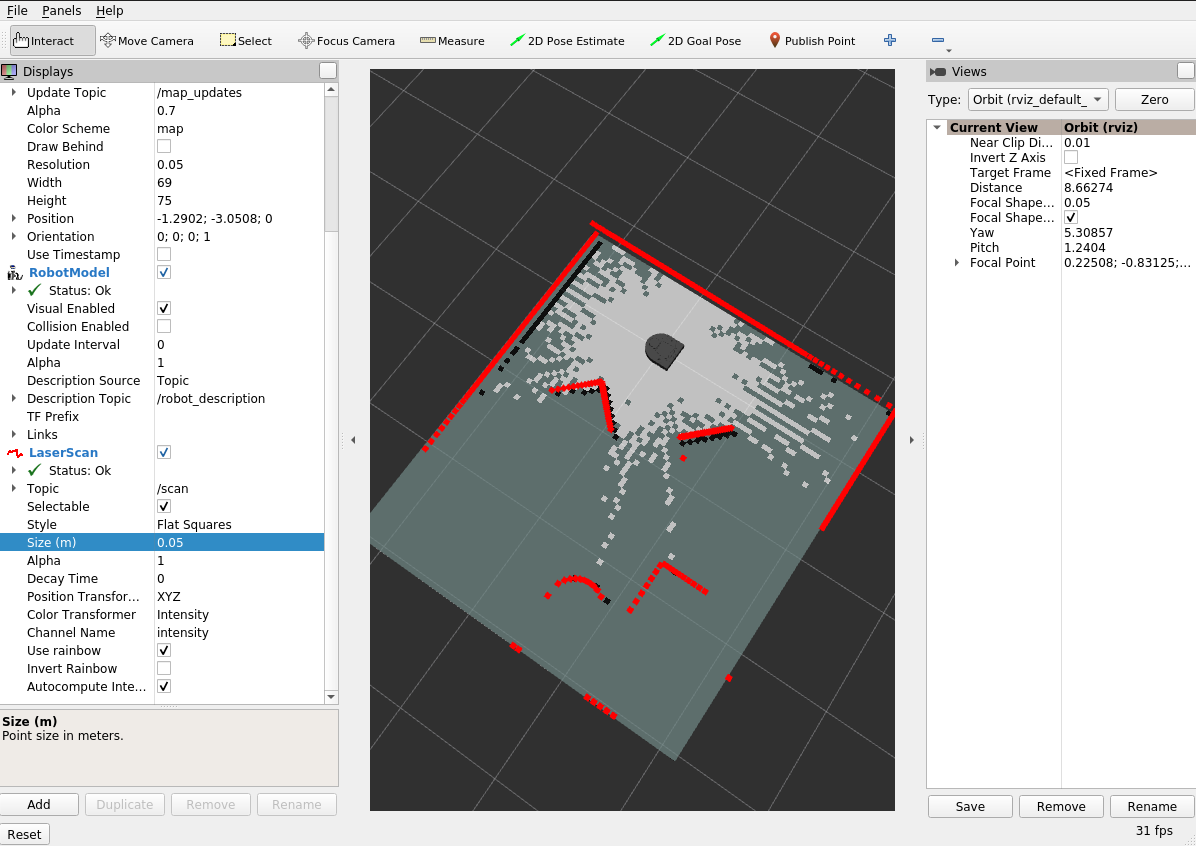
The representation of the map you see above is called an occupancy grid. The light gray spaces are mapped free space (no obstacle), the black squraes are mapped obstacles, and the dark gray space is unknown. Drive around for a while until you are able to fill in the dark gray regions.
You can now save the map using the following command (replace map_name with whatever you want to call the map).
ros2 service call /slam_toolbox/save_map slam_toolbox/srv/SaveMap "name:
  data: 'map_name'"
Make sure you can find the .yaml file that was saved in the previous step. Counterintuitively, the map is saved based on the directory you were in when you launched the slam_toolbox.
Running AMCL
Now that you have a map, you will use the built-in particle filter package called AMCL (adaptive monte carlo localization).
Before you start this step here are a few things to do.
- Stop the
slam_toolboxnodes you were running from before. Find the terminal where you ran theslam_toolbox online_sync_launch.pycommand and hitcontrol-c. - Make sure
rvizis running and load the configuration underrobot_localization/rviz/amcl.rviz(this will greatly simplify the visualization of the topics). You can use the following shortcut to make sure the configuration is loaded (note: you would have to modify this a bit if your repo is in a different location).rviz2 -d ~/ros2_ws/src/robot_localization/rviz/amcl.rviz - Make sure you know the path to the
.yamlfile created when you called the ros servicesave_map. Counterintuitively, the map is saved based on the directory you were in when you launched theslam_toolbox. Hopefully, that information will help you locate the.yamlfile. NOTE: when you use this path in the step below, you will need to replace the~character with the actual path to your home directory, e.g.,/home/pruvolo.
To start AMCL, run the following launch file.
ros2 launch robot_localization test_amcl.py map_yaml:=path-to-your-yaml-file
Make sure to replace path-to-your-yaml-file with the path you determined in step (3) of the checklist above.
Once you execute this step, if everything went well you should see output like the following.
[INFO] [launch]: All log files can be found below /home/pruvolo/.ros/log/2022-09-22-09-39-47-435007-pruvolo-Precision-3551-77054
[INFO] [launch]: Default logging verbosity is set to INFO
[INFO] [lifecycle_manager-3]: process started with pid [77060]
[INFO] [map_server-1]: process started with pid [77056]
[INFO] [amcl-2]: process started with pid [77058]
[lifecycle_manager-3] [INFO] [1663853987.576642611] [lifecycle_manager]: Creating
[lifecycle_manager-3] [INFO] [1663853987.583821848] [lifecycle_manager]: Creating and initializing lifecycle service clients
[lifecycle_manager-3] [INFO] [1663853987.587494816] [lifecycle_manager]: Starting managed nodes bringup...
[lifecycle_manager-3] [INFO] [1663853987.587568598] [lifecycle_manager]: Configuring map_server
[map_server-1] [INFO] [1663853987.592560333] [map_server]:
[map_server-1] 	map_server lifecycle node launched.
[map_server-1] 	Waiting on external lifecycle transitions to activate
[map_server-1] 	See https://design.ros2.org/articles/node_lifecycle.html for more information.
[map_server-1] [INFO] [1663853987.592774423] [map_server]: Creating
[map_server-1] [INFO] [1663853987.593316845] [map_server]: Configuring
[map_server-1] [INFO] [map_io]: Loading yaml file: /home/pruvolo/ros2_ws/src/robot_localization/maps/gauntlet.yaml
[map_server-1] [DEBUG] [map_io]: resolution: 0.05
[map_server-1] [DEBUG] [map_io]: origin[0]: -1.29
[map_server-1] [DEBUG] [map_io]: origin[1]: -3.07
[map_server-1] [DEBUG] [map_io]: origin[2]: 0
[map_server-1] [DEBUG] [map_io]: free_thresh: 0.25
[map_server-1] [DEBUG] [map_io]: occupied_thresh: 0.65
[map_server-1] [DEBUG] [map_io]: mode: trinary
[map_server-1] [DEBUG] [map_io]: negate: 0
[map_server-1] [INFO] [map_io]: Loading image_file: /home/pruvolo/ros2_ws/src/robot_localization/maps/gauntlet.pgm
[map_server-1] [DEBUG] [map_io]: Read map /home/pruvolo/ros2_ws/src/robot_localization/maps/gauntlet.pgm: 70 X 76 map @ 0.05 m/cell
[amcl-2] [INFO] [1663853987.598347033] [amcl]:
[amcl-2] 	amcl lifecycle node launched.
[amcl-2] 	Waiting on external lifecycle transitions to activate
[amcl-2] 	See https://design.ros2.org/articles/node_lifecycle.html for more information.
[lifecycle_manager-3] [INFO] [1663853987.598362596] [lifecycle_manager]: Configuring amcl
[amcl-2] [INFO] [1663853987.598468168] [amcl]: Creating
[amcl-2] [INFO] [1663853987.601084411] [amcl]: Configuring
[amcl-2] [INFO] [1663853987.601158005] [amcl]: initTransforms
[amcl-2] [INFO] [1663853987.607943895] [amcl]: initPubSub
[amcl-2] [INFO] [1663853987.611039253] [amcl]: Subscribed to map topic.
[lifecycle_manager-3] [INFO] [1663853987.613411596] [lifecycle_manager]: Activating map_server
[map_server-1] [INFO] [1663853987.613516990] [map_server]: Activating
[amcl-2] [INFO] [1663853987.613694605] [amcl]: Received a 70 X 76 map @ 0.050 m/pix
[lifecycle_manager-3] [INFO] [1663853987.613789388] [lifecycle_manager]: Activating amcl
[amcl-2] [INFO] [1663853987.613883938] [amcl]: Activating
[amcl-2] [WARN] [1663853987.613896432] [amcl]: Publishing the particle cloud as geometry_msgs/PoseArray msg is deprecated, will be published as nav2_msgs/ParticleCloud in the future
[lifecycle_manager-3] [INFO] [1663853987.614092632] [lifecycle_manager]: Managed nodes are active
[amcl-2] [INFO] [1663853987.751946277] [amcl]: createLaserObject
[amcl-2] [WARN] [1663853989.757340775] [amcl]: ACML cannot publish a pose or update the transform. Please set the initial pose...
[amcl-2] [WARN] [1663853991.764180749] [amcl]: ACML cannot publish a pose or update the transform. Please set the initial pose...
The last line where AMCL is complaining about wanting an initial pose, brings us to our next step. Go to rviz2 (make sure you loading the .rviz configuration specified above) and set an initial location for the particle filter using the 2D Pose Estimate Widget. Click the location in the map where you think the robot is and drag in the direction you think the robot is facing. Once you release the mouse, the visualizations of your robot and your LIDAR should return. You should also see a bunch of red arrows indicating the particle locations. Drive around for a while and see if the AMCL is able to converge to the correct robot pose. How do you know if it is correct or not? Here is an example of how it might look (note: despite my best efforts, I picked a bad initial position for AMCL. Despite this, it was able to eventually figure out where the robot was).
Localizing a Robot
Return to the terminal where the rosbag is playing and click space bar. Return to rviz. You should see a cloud of particle in the map that move around with the motion of the robot. If you want the particle filter to work well, you can update the 2D pose estimate based on the arrow shown by the map_pose topic. If all goes well, you’ll see the robot moving around in the map and the cloud of particles condensing to the true pose of the robot.
Running your own Particle Filter
The instructions for running your particle filter are identical except for you need to use a different launch file to startup your code.
ros2 launch robot_localization test_pf.py map_yaml:=path-to-your-yaml-file
Localization with Bag Files
We have included some bag files in the repository that you can use to work on the project. The bag files included are in the following locations. These bag files have been collected from the Turtlebot4.
robot_localization/bags/macfirst_floor_take_1
robot_localization/bags/macfirst_floor_take_2
Each bag file corresponds to the map.
robot_localization/maps/mac_1st_floor_final.yaml
Note: before doing this, make sure Gazebo is shutdown and you are not connected to a physical robot (remember, the bag file will be supplying the sensor data)
ros2 bag play path-to-your-bag-file --clock
In order to test your particle filter (pf.py) with a bag file, you can start up the particle filter as before.
ros2 launch robot_localization test_pf.py map_yaml:=path-to-your-yaml-file
Note 1: You’ll see that we are instructing our code to avoid using the simulator time (since this data is from a real robot). Note 2: Currently, I am not able to make the bag files work with the built-in particle filter. This is not a big deal since we are coding our own, but it’s worth noting.
The setup for rviz is pretty involved, so we have provided a configuraion file for you. Once rviz is open, you can click File then Open Config and the select ~/ros2_ws/src/robot_localization/rviz/turtlebot_bag_files.rviz.
Alernatively, you can launch rviz2 and pass the configuration file on the command line.
rviz2 -d ~/ros2_ws/src/robot_localization/rviz/turtlebot_bag_files.rviz
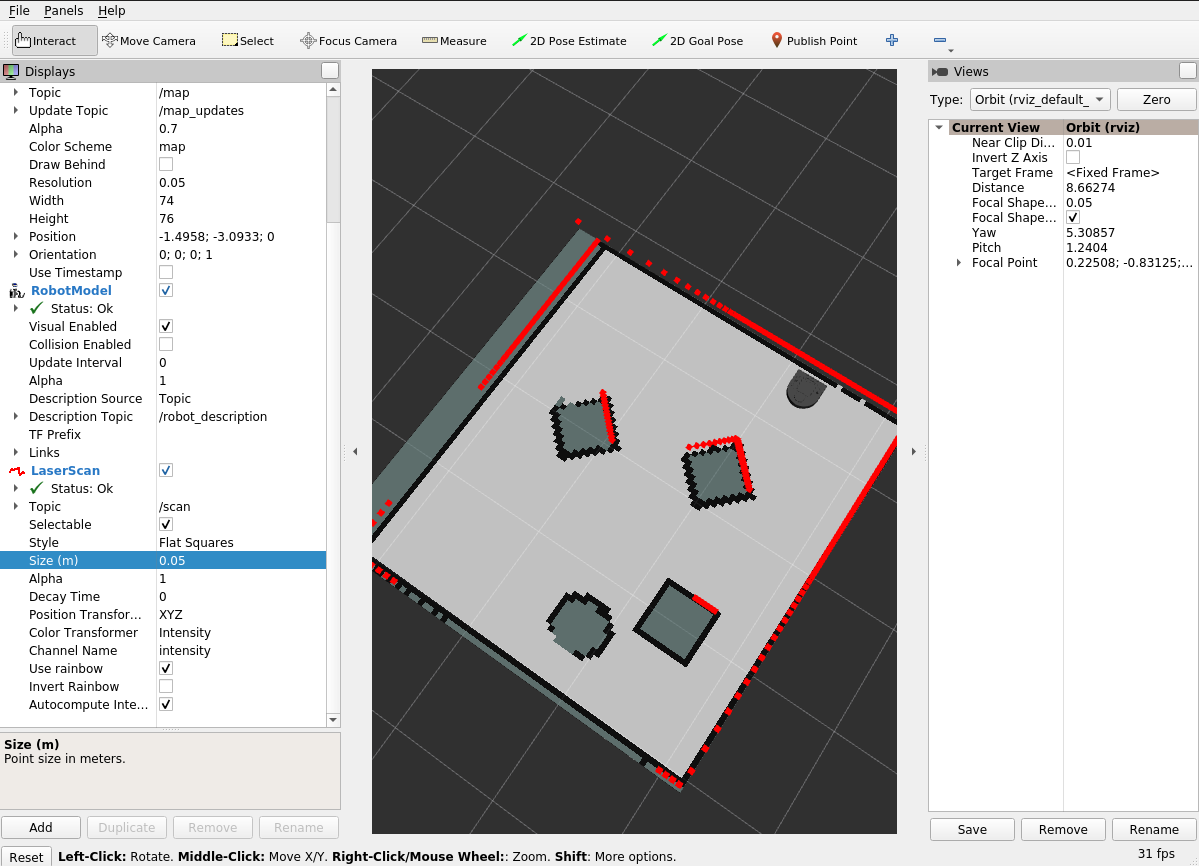
As with testing live, you will need to set an initial pose with the 2D Pose Estimate in rviz. As the bag plays you will see the robot move around in the map in rviz. If your particle filter has localized your robot properly, the laser scans will line up with the features of the map.
When the bag is finished playing, you will probably want to perform the following steps to try another run of the particle filter.
- Reset rviz by clicking the
resetbutton. - Restart your particle filter by launching
test_pf.py. - Restart the bag file via
ros2 bag play.
Recording your own bag files
You can make your own bag files either with the physical robot or the simulator. When recording a bag file of the Neato, you’ll want to modify your recording command a bit from what you did in the warmup project.
ros2 bag record /accel /bump /odom /cmd_vel /scan /robot_description /stable_scan /projected_stable_scan /clock /tf /tf_static -o bag-file-name-here
Choosing Your Own Adventure and Going Beyond
You have complete latitude for choosing your approach to particle filtering. While we’ve provided some skeleton code and reference AMCL in this project, there are many other particle-filtering or state-estimation techniques that you can examine. We highly recommend searching Google Scholar, StackOverflow, or the ROS2 Forums for some inspiration; you might also consider:
- How you might modify or expand upon one key step of the particle filter to enhance speed, memory, or robustness (e.g., hierarchical sampling, adaptive particle counts, partial-map references, etc.).
- Experimenting with “ambiguous scenarios” or different initialization schemes.
- Experimenting with different quality of laser data (adding noise to simulated inputs, using the vehicle, etc.) and analyzing uncertainty in your filter.
- Implementing different filtering techniques, based on optimization schemes (e.g., Kalman Filtering, Extended Kalman Filtering, etc.).
- Considering how different robot behaviors may impact localization quality.
- Attempting to implement a bare-bones SLAM (simultaneous localization and mapping) pipeline (or running an open-source technique and comparing it to your localization-only technique).
Project Advice
Instructor Advice
- Use the provided rosbags to debug your code (or, for practice, make your own ROS bags)
- Visualize as many intermediate computations as possible
- Start with simple cases, e.g. start with just one particle, make sure you can visualize the particle in rviz
- Build test cases that can be used to assess that snippets/functions of your code are working as expected. You can use a bag-file you collect within a test case as well.
- Implement a simple laser scan likelihood function. Test it using just a subset of the Lidar measurements. Make sure that the results conform to what you expect (the simulator or rosbag will be helpful here).
- Improve your laser scan likelihood to maximize performance. Again, rosbag and visualization will be instrumental here.
Previous Student Advice
Here is some advice from the Fall 2018 class that they wrote up after they completed the robot localization project.
- Pixels vs meters on map (know how these relate to each other)
- Know how coordinate frames relate to one another on rviz displays
- Know what the different rviz topics represent
- Probabilistic justification for parameters (and then cube it for good measure)
- High level understanding (videos) were helpful +1 +1
- Visualization in rviz is crucial
- First pass architecture (should be evaluated / given feedback) (note: this is more of a suggestion for the teaching team than you all).
- Maybe should have done a “ugly, rugged thing” would have helped to get an MVP. Maybe a more iterative process rather than strict planning. All the objects we created were hard to glue together.
- Take a “second pass” at the architecture after attempting to implement your first one. Take a step back and ask what you would do differently after having grappled with the low-level code for a week.
- Test each step of the particle filter separately, with full rviz visualizations, with single particles. Create a testing plan!
- Creativity in the weighting algorithm was nice since the x/y distance helper function just worked
- Rosbags are wonderful, wonderful things +1000
- Possibly some more scaffold around researching what amcl does and pull from it to test each part of the filter
Resources
- Video Explaining Particle Filter without Equations
- An Example of a Particle Filter that Might Give More Intuition
- Very Mathy / Theoretical Treatment of Particle Filter (not for the faint of heart, but we can help you through it)
- A good high-level overview with some great visualizations: Autonomous Navigation: Understanding the Particle Filter